Are you tired of scrolling endlessly in your Google Sheets to find important information? Look no further!
In this article, we will show you how to freeze a row in Google Sheets. By following our step-by-step guide, you’ll be able to keep your headers or any important data in view while you navigate through your spreadsheet.
Say goodbye to tedious scrolling and hello to an efficient and organized workflow. Let’s get started!
Understanding the Importance of Freezing Rows
Understanding the importance of freezing rows can greatly enhance your productivity in Google Sheets. When working with large datasets or lengthy spreadsheets, it can become challenging to keep track of important information while scrolling through rows.
By freezing rows, you can ensure that the headers or key data points remain visible at all times, even when you’re working with a lot of data. This allows for easy reference and prevents the need to repeatedly scroll back up to the top.
Imagine how much time and effort you can save by simply freezing the rows that contain crucial information. It not only improves your efficiency but also allows you to focus on analyzing and manipulating the data without any distractions.
Step-by-Step Guide to Freezing a Row in Google Sheets
To start, let’s take a look at how you can easily keep a specific row visible while scrolling through your document in Google Sheets.
This feature, known as ‘freezing’ a row, is incredibly helpful when you have a large dataset and want to keep important information, like headers, always visible.
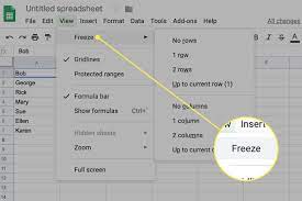
To freeze a row in Google Sheets, simply select the row you want to freeze by clicking on the row number, right-click, and choose ‘Freeze’. Alternatively, you can go to the ‘View’ menu, select ‘Freeze’, and then choose ‘1 row’.
Once you’ve done this, the frozen row will stay at the top of your screen as you scroll through the rest of your document, ensuring that you never lose sight of important data.
Exploring Different Methods to Freeze Rows in Google Sheets
When using Google Sheets, there are various techniques available for keeping a specific row visible while scrolling through your document.
One method is to use the ‘Freeze’ feature. To do this, simply click on the row number or select the entire row, then go to the ‘View’ menu and click on ‘Freeze.’
Another method is to use the ‘Split’ feature. To do this, click on the desired row number, then go to the ‘View’ menu and click on ‘Split.’ This will split your sheet into two sections, with the selected row remaining visible at the top.
You can also use the ‘Filter’ feature to freeze a specific row. Just click on the filter arrow in the row you want to freeze, and then select ‘Filter by condition’ and choose a condition that will keep the row visible.
With these techniques, you can easily keep a specific row visible while scrolling through your Google Sheets document.
Troubleshooting Common Issues When Freezing Rows in Google Sheets
One common issue you may encounter is difficulty in keeping a specific section visible while scrolling through your document in Google Sheets. This can be frustrating when you’re working with large datasets and need to refer back to certain rows or columns frequently.
Luckily, there is a simple solution to this problem. By freezing rows or columns, you can ensure that they remain visible even when you scroll through the rest of your sheet.
To freeze a row, simply select the row below the one you want to freeze, then go to the ‘View’ menu and click on ‘Freeze’ followed by ‘Up to current row.’
Similarly, you can freeze columns by selecting the column to the right of the one you want to freeze and choosing ‘Freeze’ and ‘Up to current column’ from the ‘View’ menu.
Advanced Tips and Tricks for Freezing Rows in Google Sheets
If you’re working with large datasets in Google Sheets, it’s helpful to freeze certain sections to keep them visible while scrolling.
One advanced tip for freezing rows in Google Sheets is to freeze multiple rows at once. To do this, simply select the row below the last row you want to freeze, right-click on the selected row, and choose ‘Freeze rows X-X’ from the dropdown menu.
Another useful trick is to freeze rows and columns simultaneously. To achieve this, select the cell below the last row you want to freeze and to the right of the last column you want to freeze. Then, right-click on the selected cell, go to ‘Freeze’, and choose the appropriate option from the list.
These advanced techniques can greatly enhance your data analysis experience in Google Sheets.
Conclusion
In conclusion, freezing rows in Google Sheets is a valuable feature that can greatly enhance your spreadsheet organization and navigation. By following the step-by-step guide and exploring different methods, you can easily freeze rows to keep important information visible as you scroll.
If you encounter any issues, the troubleshooting section can help you overcome them. Additionally, the advanced tips and tricks can further optimize your freezing experience.
With these techniques, you’ll be able to efficiently manage your data and improve your productivity in Google Sheets.